[Econometrics] Econometrics in Python
파이썬에서 계량분석에 대해 어떤 기본적인 라이브러리가 있고, 어떻게 쓰면 되는지 간단한 팁들을 작성해보려 합니다.
- Patsy: 데이터 전처리와 같은 작업
- Statsmodels: 횡단면 및 시계열 데이터 분석
- Linearmodels: 패널데이터 분석
- Stargazer: 결과 서머리표 (관리가 잘 안되고 있으며 Linearmodels는 지원 하지 않음)
Visualization style
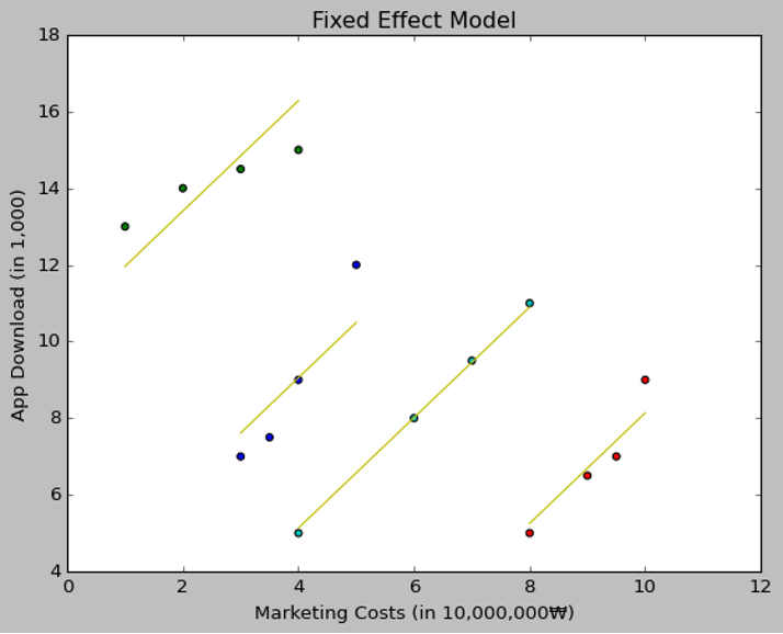
리서치 페이퍼, 리포트 등의 용도로 정적인 시각화를 할 때 가장 클래식한 기본 그래프 스타일은 다음과 같이 표현합니다.
(참고 matplotlib )
from matplotlib import style
from matplotlib import pyplot as plt
%matplotlib inline
plt.style.use(["classic"])

plt.plot(color="C5")
예시코드 및 결과
plt.scatter(toy_panel.mkt_costs, toy_panel.app_download, c=toy_panel.city)
for city in fe_toy["city"].unique():
    plot_df = fe_toy.query(f"city=='{city}'")
    plt.plot(plot_df.mkt_costs, plot_df.y_hat, color ="C5")

plt.title("Fixed Effect Model")
plt.xlabel("Marketing Costs (in 10,000,000₩)")
plt.ylabel("App Download (in 1,000)")
Data prep using patsy
patsy 는 statistical model을 묘사하기 위한 python package 이며 R-style formula로 Y ~ x1 + x2 처럼 선형적인 관계를 symbolic 하게 표현해주며 또한 문자열로 되어있는 범주형 컬럼도 더미변수화 해줍니다. statsmodels 나 linearmodels 를 사용할 때 직관적인 high-level interface를 제공합니다.
import numpy as np
import pandas as pd
from patsy import dmatrix
from patsy import demo_data

df = pd.DataFrame(demo_data("x1","x2","x3","x4"))

def mean_diff(x):
	return x - np.mean(x)

#기본 API
dmatrix(formula_like, data={}, eval_env=0, NA_action='drop', return_type='matrix')
#NA_action: null값 어떻게 할건지 "drop" or "raise" an error
#return_type: "matrix" or "dataframe"

# 예시에선 상수항도 표현하기 위해 + 1 을 하였지만 더미변수를 넣는다면 축소랭크 방식(카테고리 변수 n-1)으로 하므로 + 1 생략할것
dmatrix("x1 + mean_diff(x2) + np.log(x3) + x1:x2 + I(x1+x2) + C(x4) + 1",
 data=df)

# 카테고리변수 더미화(축소랭크) 예시
dmatrix("C(X1) + Y", data=df, return_type='dataframe')
# baseline 값을 바꾸고 싶다면
dmatrix("C(X1, Treatment('카테고리1')) + Y", data=df, return_type='dataframe')
표현 방법 설명
1: 상수항 (기입하지 않아도 알아서 들어감 만약 상수항을 넣기 싫다면 -1) 즉, y ~ x1 -1y ~ x1이여도 default 로 상수항이 있는y ~ 1 + x1이긴합니다
:: interaction term- interaction term과 변수를 한번에 표현하려면?
*즉,x1 + x2 + x1:x2=x1*x2
- interaction term과 변수를 한번에 표현하려면?
I(): interaction 을 제외하고는I()라는 연산자를 사용하여 연산자를 명시해야 함 (예시는 x1컬럼과 x2컬럼의 합)- 함수를 넣어 변수 변환 가능
- ex)
np.log(),np.log1p()직접만든mean_diff()
- ex)
- 이 외에도 스케일링 작업을 위한 함수도 제공합니다
center(): 평균을 0으로 스케일링 (mean_diff와 같음)standardize(): 평균을 0으로 하고 표준편차를 1로 스케일링- 스케일링을 했던 평균값 등은
design_info.factor_infos에 저장됩니다 → 통계분석에선 상관없지만 예측모형에선 모형을 학습할 때 사용한 것과 동일한 전처리(새로운 데이터에도 똑같은 기존에 맞게 똑같이 처리를 해줘야함)를 해야하기 때문입니다.
C(): 데이터가 범주형 값이지만 정수로 표시된 경우 C()를 이용해 categorical variable로 지정Treatment(): baseline값 변경 원할시 dmtrix(“C(x, Treatment(‘category1’))”, df)- 결과값에 컬럼명이 T. 인건 treatment coded 라는 뜻입니다.
- 여러개의 범주형 변수가 있는 경우
- 통합 축소형: dmatrix(”x1+x2”) 와 같이하며 더미변수는 변수의 갯수와 상관없이 하나로 통합합니다.
Modules for statistical analysis
python에서 통계적인 모델링은 statsmodels, linear models 를 주로 사용하며 구현되지 않은 방법론(Tobit, Heckit, PSM, IPW 등)은 따로 이를 이용해 만들거나 따른 모듈을 찾아서 써야합니다. 저 같은 경우는 직접 구현해보거나 다른 모듈의 소스코드를 확인 후 사용합니다.
Statsmodels
formula style을 사용하는 기본적인 방법은 다음과 같습니다.
import statsmodels.formula.api as smf
# smf.gls ,smf.wls , smf.ols, smf.glm 등 api를 다 소문자로 하면 됩니다.
mod = smf.ols(formula='players ~ Action + Indie + Strategy + Adventure + Casual',
              data=pd.concat([u_treat_group,u_control_group]))
res = mod.fit()
print(res.summary())

# logit
mod = smf.logit(formual = "Treated", dafa=df)
res = mod.fit()
# odds ratio for dummy variable
np.exp(res.params)
# marginal effects
res.get_margeff(at='mean').summary() # mean or overall

# GLM model (Binomial)
mod1 = smf.glm(formula=formula, data=dta, family=sm.families.Binomial()).fit()
print(mod1.summary())
Linearmodels
panel data를 다룰때 Linearmodels를 사용하면 간편합니다.
import linearmodels as lm

formula = f"Treated ~ value + market_share + price + discount_rate + 1 + EntityEffects + TimeEffects"

mod = lm.PanelOLS.from_formula(formula, data=pd.concat([treat_group,control_group]).set_index(['appid',"time_index"]), drop_absorbed=True)
res = mod.fit(cov_type='clustered')
res.summary
모델의 결과물들
result = model.fit() 을 통해 나오는 결과물들은 dir(result)로 확인 가능합니다. log-level, log-log 등 모형에서 더미변수의 해석, logit에서의 회귀계수 해석등을 더 쉽게 하려면 회귀 결과물에서 따로 빼와 exp()을 취하는 등 계산을 해야해서 알아두면 편합니다.
res. summaryres. summary2res.pvalues res. params: 회귀계수res. bse: std_errres. conf_intrsquared rsquared_adj f_pvalue df_model: degree_freedom df_resid: degree_freedom_resid nobs: number of obs fvalue: f_statistic
Standard Errors
회귀분석시 Heteroskedasticity 와 Autocorrelation 을 고려하기 위한 standard errors 계산 코드 예시입니다.
import numpy as np
import pandas as pd
import statsmodels.formula.api as smf
import statsmodels as sm
import linearmodels as lm

# simple ols use_t for use t-statistics to compute the p-value
ols = smf.ols(formula='y ~ x', data=df).fit(use_t=True)

# adding heteroscedasticity-consistent standard errors
# HCO(the original white estimator) ~ HC3
robust_ols = smf.ols(formula='y ~ x', data=df).fit(cov_type='HC1', use_t=True)

# OLS Coefficients and Standard Errors Clustered by Firm or Year
cluster_firm_ols = smf.ols(formula='y ~ x', data=df).fit(cov_type='cluster',
                                                        cov_kwds={'groups': df['firmid']},
                                                        use_t=True)
# 2way cluster
cluster_2ways_ols = smf.ols(formula='y ~ x', data=df).fit(cov_type='cluster',
                                                         cov_kwds={'groups': np.array(df[['firmid', 'year']])},
                                                         use_t=True)
# Fixed effects
# linearmodels needs the index to be entity/date.
df2 = df.set_index(['firmid', 'year'])
# two-way fixed effects
firm_year_fe_panel = lm.PanelOLS.from_formula('y ~ x + EntityEffects + TimeEffects', data=df2).fit()
# Standard Errors clustered in panel data with two-way fixed effects
res = lm.PanelOLS.from_formula('y ~ x + EntityEffects + TimeEffects', data=df2).fit(cov_type='clustered', cluster_entity=True, cluster_time=True)

# statsmodel 로 fixed efffects 구현하려면 카테고리 C 사용하며 더미들을 만들 수 있으나 linearmodels쓰는게 편함
firm_year_fe_ols = sm.ols(formula='y ~ x + C(firmid) + C(year)', data=df).fit(use_t=True)

# Newey-West Adjustment for Standard Errors
# (heteroskedasticity and autocorrelation consistent)
nw_ols = smf.ols(formula='y ~ x', data=df).fit(cov_type='HAC',
                                              cov_kwds={'maxlags': 3},
                                              use_t=True)
# Driscoll-Kraay Standard Errors for panel data
dk_ols = smf.ols(formula='y ~ x', data=df).fit(cov_type='nw-groupsum',
                                              cov_kwds={'time': np.array(df.year),
                                                        'groups': np.array(df.firmid),
                                                        'maxlags': 5},
                                              use_t=True)
Report regression output
stata 의 outreg2 나 R의 stargazer 처럼 descriptive statistics 나 분석결과를 엑셀, latex 등으로 해주는 패키지가 파이썬은 빈약합니다.
R의 stargazer 을 implement한 python의 stargazer가 있지만 statsmodels의 결과만 가져올 수 있고, output으로 excel 형태는 불가능 합니다. 즉, 직접 코드를 짜거나 수정 해야합니다.
import pandas as pd
from sklearn import datasets
import statsmodels.api as sm
from stargazer.stargazer import Stargazer

diabetes = datasets.load_diabetes()
df = pd.DataFrame(diabetes.data)
df.columns = ['Age', 'Sex', 'BMI', 'ABP', 'S1', 'S2', 'S3', 'S4', 'S5', 'S6']
df['target'] = diabetes.target

est = sm.OLS(endog=df['target'], exog=sm.add_constant(df[df.columns[0:4]])).fit()
est2 = sm.OLS(endog=df['target'], exog=sm.add_constant(df[df.columns[0:6]])).fit()

# stargazer 를 불러온뒤 각 결과 객체를 감싸면 됨
stargazer = Stargazer([est, est2])
# custom title 제목
stargazer.title('분석 study')

# custom model names 모델 이름 커스텀
stargazer.custom_columns(['Model1 LPM','Model2 Logit'],[1,1])
# Subset Covariates and/or Choose Covariate order 변수 순서 설정
stargazer.covariate_order(['BMI','Age','Sex'])
# Rename Covariates 변수 이름 변경
stargazer.rename_covariates({'Age':'Oldness'})

# Show Custom Notes 맨밑에 노트 추가
stargazer.add_custom_notes(['First note','Second note'])
# Add Custom Lines 설명줄 추가
stargazer.add_line('More controls',['No','No'])
stargazer.add_line('Preferred',['No','Yes'], LineLocation.FOOTER_TOP)

# remove model numbers 모델번호 제거
stargazer.show_model_numbers(False)
# Hide/Show Degrees of Freedom
stargazer.show_degrees_of_freedom

# 결과 html로
stargazer.render_html()
# 결과 latex로
stargazer.render_latex()

# html to csv 완벽하진 않으나 엑셀에 결과 옮기기 가장 쉬움
with open('result.html','w') as f:
	f.write(stargazer.render_html())
result = pd.read_html('result.html')
result[0].to_csv('result.csv')